I've spent more years than I care to remember analysing vegetation survey data (typically species abundances in plots) using a variety of software including my own algorithms coded in FORTRAN and C++. A recent query on the r-help list, about how to determine the number of groups to define in a hierarchical classification produced with the hclust function, prompted me to unearth one of these algorithms, homogeneity analysis1, which can help to visualize how different levels of grouping partition the variability in a distance matrix.
This algorithm is extremely simple. The classification is progressively divided into groups, with all groups being defined at the same dendrogram height. At each level of grouping, the average of within-group pairwise distances is calculated. Homogeneity is then defined as:
where Davtotal is the average pairwise distance in the dataset as a whole.
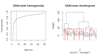
For data were there exist well-defined clusters of values, a plot of homogeneity against number of groups will display an 'elbow' where the initial rapid increase in homogeneity turns to a more gradual increase. The example above shows a classification of the USArrests dataset and corresponding homogeneity plot which suggests defining 7 groups. It was generated as follows:
Here is the code for the hmg function:
Reference
1M. Bedward, D. A. Keith, R. L. Pressey. 1992. Homogeneity analysis: Assessing the utility of classifications and maps of natural resources. Australian Journal of Ecology 17(2) 133-139.

This algorithm is extremely simple. The classification is progressively divided into groups, with all groups being defined at the same dendrogram height. At each level of grouping, the average of within-group pairwise distances is calculated. Homogeneity is then defined as:
H = 1 - Davwithin-group - Davtotal
where Davtotal is the average pairwise distance in the dataset as a whole.
For data were there exist well-defined clusters of values, a plot of homogeneity against number of groups will display an 'elbow' where the initial rapid increase in homogeneity turns to a more gradual increase. The example above shows a classification of the USArrests dataset and corresponding homogeneity plot which suggests defining 7 groups. It was generated as follows:
> d <- dist(USArrests)
> hc <- hclust(d, method="average")
> h <- hmg(d, hc)
> plot(h, type="s", main="USArrests homogeneity")
> abline(v=7, lty=2)
> plot(hc, labels=FALSE, main="USArrests dendrogram")
> rect.hclust(hc, k=7)
Here is the code for the hmg function:
function(d, hc) {

# R version of homogeneity analysis as described in:
#   Bedward, Pressey and Keith. 1992. Homogeneity analysis: assessing the
#   utility of classifications and maps of natural resources
#   Australian Journal of Ecology 17:133-139.
#
# Arguments:
# d  - either an object produced by dist() or a vector of
#      pairwise dissimilarity values ordered in the manner of
#      a dist result
#
# hc - classification produced by hclust()
#
# Value:
# A two column matrix of number of groups and corresponding homogeneity value
#
# This code by Michael Bedward, 2010

  m <- hc$merge

  # check args for consistency
  Nobj <- nrow(m) + 1
  if (length(d) != Nobj * (Nobj-1) / 2) {
    dname <- dparse(substitute(d))
    hcname <- dparse(substitute(hc))
    stop(paste(dname, "and", hcname, "refer to different numbers of objects"))
  }

  distMean <- mean(d)
  grp <- matrix(c(1:Nobj, rep(0, Nobj)), ncol=2)

  # helper function - decodes values in the merge matrix
  # from hclust
  getGrp <- function( idx ) {
    ifelse( idx < 0, grp[-idx], getGrp( m[idx, 1] ) )
  }

  grpDistTotal <- numeric(Nobj)
  grpDistCount  <- numeric(Nobj)
  hmg <- numeric(Nobj)
  hmg[1] <- 0
  hmg[Nobj] <- 1

  distTotal <- 0
  distCount <- 0
  for (step in 1:(Nobj-2)) {
    mrec <- m[step, ]
    grp1 <- getGrp(mrec[1])
    grp2 <- getGrp(mrec[2])

    distTotal <- distTotal - grpDistTotal[grp1] - grpDistTotal[grp2]
    distCount <- distCount - grpDistCount[grp1] - grpDistCount[grp2]

    grpDistTotal[grp1] <- grpDistTotal[grp1] + grpDistTotal[grp2]
    grpDistCount[grp1] <- grpDistCount[grp1] + grpDistCount[grp2]

    grp1Obj <- which(grp == grp1)
    grp2Obj <- which(grp == grp2)

    for (i in grp1Obj) {
      for (j in grp2Obj) {
        ii <- min(i,j)
        jj <- max(i,j)
        distIdx <- Nobj*(ii-1) - ii*(ii-1)/2 + jj-ii
        grpDistTotal[grp1] <- grpDistTotal[grp1] + d[distIdx]
        grpDistCount[grp1] <- grpDistCount[grp1] + 1
      }
    }

    # update group vector
    grp[grp == grp2] <- grp1

    distTotal <- distTotal + grpDistTotal[grp1]
    distCount <- distCount + grpDistCount[grp1]

    hmg[Nobj - step] <- 1 - distTotal / ( distCount * distMean )
  }

  out <- matrix(c(1:Nobj, hmg), ncol=2)
  colnames(out) <- c("ngroups", "homogeneity")
  out
}
Reference
1M. Bedward, D. A. Keith, R. L. Pressey. 1992. Homogeneity analysis: Assessing the utility of classifications and maps of natural resources. Australian Journal of Ecology 17(2) 133-139.
Hi Michael,
ReplyDeleteexcellent post, thanks, it actually helps me with my current work. Would you know of a nice (?simple) way to automatically determine the number of the groups, not by pure visual assessment?
Thanks,
Martin
Hi Martin,
ReplyDeleteOne simple way (a fudge really) is to try to detect when the slope of the curve is more or less constant for a while, indicating that you (could) have passed the 'elbow' (if there was one). If the slope is constant-ish the second derivative will be near zero for successive points. The following function attempts to do this...
function( h, tol=0.02, npoints=3 ) {
d2 <- diff(h[,2], 1, 2)
for (i in 1:(length(d2)-npoints)) {
if (all(abs(d2[i:(i+npoints)]) <= tol)) {
return(i+2)
}
}
cat("bummer - failed")
NULL
}
If you try that out let me know how you go. Keep in mind that it is definitely a "rough" method :)
another idea would b to look for the point of max curvature (would probably first need to smooth the graph).
ReplyDeletehttp://www.intmath.com/applications-differentiation/8-radius-curvature.php
What do you reckon?
Hi Martin,
ReplyDeleteYes that might be useful, though I suspect it would be more fiddly than the constant slope approach. It would probably also be a good idea to exclude the last portion of the curve which often has a kick upwards as you approach all groups being singletons.
Another idea that might be worth mentioning: you could 'test' (in a loose sense) the usefulness of splitting a group into two child groups via a monte carlo procedure where you randomly allocate objects from the parent group to the child groups and compare the average within group distance to the 'real' child groups. I might do a post on that to illustrate the idea.
Hi Michael,
ReplyDeleteI have tried it with both approaches (mine, radius based, and yours, slope based, the results are similar, although not identical, depending on a few parameters.). Is it ok if I email (would use your contact from the geotools mailing list, if that's ok) you the pdf with printouts and the code? I am not sure how I would put it here. If you think it's interesting, feel free to put it then to your blog.
Cheers
Martin
Hi Martin,
ReplyDeleteGeoTools ? Small world :)
Yes please email me - I'd like to have a look.
cheers
Michael